

Overview
INTRODUCTION
Dirty data are everywhere. In fact most real world dataset start off dirty in one way or another. By the time they made their way in textbook and course, most are already been cleaned and prepared for analysis. This is really convenient when all you want to talk about is how to analyze or model the data. But it can leave you a loss when you face cleaning your own data. Also the thrive of (so-called) big data, data cleaning is more important than ever before. And the data get bigger, the number of things go wrong do too. Each imperfection become harder to find that we cannot really look at the entire dataset and the spreadsheet on your computer. In fact data cleaning is the central part of data science process.
Unless the data is small, the presence of incorrect and inconsitent data is pervasive. As a result, we should spend a lot of time cleaning data. This time is also, typically underestimated.
By way of showing how data is messy in real life, I used for sale vehicle data which is harvested from Craiglist. Craiglist car for sale is where the the owners and dealers create a post for a vehicle providing information about model, year of the vehicle, fuel type, how many miles there are on the odometer. Here are the description of the variables in the data:
id the (unique) identifier for the post
title a short text description for the post
body the full free-form text for the post
lat, long the longitude and latitude associated with the post, i.e., that of the poster or of the location of the car, or both.
posted the date the post was originally posted
updated the date of the most recent modification to the post
drive what type of drive the vehicle has, e.g., front-wheel drive.
odometer the number of miles on the car’s odometer
type what type of vehicle is the post about, e.g., car, van, truck.
header a shot description for the post, different from the body, and potentially different form the title.
condition a description of what condition the vehicle is in, e.g., excellent
cylinders the number of cylinders in the vehicle’s engine.
fuel the type of fuel the vehicle uses, e.g., gas
size a categorical description of the size of the vehicle, e.g., compact, mid-size.
transmission the transmission type of the vehicle, e.g., automatic, manual.
byOwner a logical value with TRUE indicating the vehicle is being sold by its owner, not a dealer
city the city on whose bulletin board the post was submitted
time the date and time when the post was posted
description a short description for the post
location the user-supplied city/town for the post
url part of the URL for the post
price the price being sought for the vehicle
year the year the car was manufactured
maker the name of the car manufacturer, e.g., ford, chevrolet. These are extracted from the header or title of the post.
makerMethod a number that identifies which method was used to identify the manufacturer
SET UP
- Loading data into R
- Use ls() to list files. Data is named as
vehicle
load("~/Dropbox/Fall 2015/STAT 141/Assignment1/vehicles.rda")
ls()
[1] "vehicle"
- Libraries are used:
library(lattice)
library(maps)
library(ggplot2)
library(gmodels)
library(RColorBrewer)
DATA EXPLORATION AND CLEANING
First, we need to examine what is the class of vehicle
> class(vehicle)
[1] "data.frame"
Since vehicle is a data frame, we need to know its dimension.
> dim(vehicle)
[1] 34677    26
vehicle dataset contains 26 variables and 34677 observations.
Even though we have already known the decription of each variable above, we should carefully confirm the names of these variables and identify its class.
> names(vehicle)
 [1] "id"           "title"        "body"         "lat"          "long"
 [6] "posted"       "updated"      "drive"        "odometer"     "type"
[11] "header"       "condition"    "cylinders"    "fuel"         "size"
[16] "transmission" "byOwner"      "city"         "time"         "description"
[21] "location"     "url"          "price"        "year"         "maker"
[26] "makerMethod"

> unlist( sapply(X = vehicle, FUN = class) )
          id        title         body          lat         long      posted1
 "character"  "character"  "character"    "numeric"    "numeric"    "POSIXct"
     posted2     updated1     updated2        drive     odometer         type
    "POSIXt"    "POSIXct"     "POSIXt"     "factor"    "integer"     "factor"
      header    condition    cylinders         fuel         size transmission
 "character"     "factor"    "integer"     "factor"     "factor"     "factor"
     byOwner         city        time1        time2  description     location
   "logical"     "factor"    "POSIXct"     "POSIXt"  "character"  "character"
         url        price         year        maker  makerMethod
 "character"    "integer"    "integer"  "character"    "numeric"
In this dataset, price is the most important variable to me. To get an in-depth look at the price variable, we should see the distribution of vehicle price.
densityplot(vehicle$price, main = "Price", xlab = "Price")
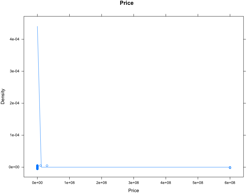
=> densityplot indicates that there are a few extreme outliers in the right tail. Let’s check them out.
> tail( sort(vehicle$price), 50)
 [1]     95593     96590     97000     97500     97911     98000     99560
 [8]     99999    100000    100000    100000    100000    104800    105000
[15]    105500    107000    112000    116100    116491    120000    122950
[22]    123981    125000    129950    129990    138500    139000    139950
[29]    143000    143000    143950    147000    149890    149995    150000
[36]    152900    159000    169000    177588    202455    240000    286763
[43]    359000    400000    559500    569500   9999999  30002500 600030000
[50] 600030000
=> Obviously, the price of a car > 9999999 is quite unlikely. Let’s take a look at them.
> idx = which( vehicle$price >=  9999999 & !is.na(vehicle$price) )
> vehicle[ idx, c("header", "price", "maker", "year") ]
                            header     price    maker year
posted22491       1969 Pontiac GTO 600030000  pontiac 1969
posted23881       1969 Pontiac GTO 600030000  pontiac 1969
posted6903  2002 Caddy Seville sls  30002500 cadillac 2002
posted16005      2001 Honda Accord   9999999    honda 2001
It is realized that those are pretty old cars => Their high prices are probably not legitimate. Let’s check and fix them:
- With Pontiac GTO :
    > idx = ( vehicle$maker == "pontiac" & vehicle$year %in% c(1968, 1969) &
+ vehicle$price < 9999999 & vehicle$price > 1 &
+ grepl(pattern = "GTO", x = vehicle$header, ignore.case = TRUE) &
+ !is.na(vehicle$maker) & !is.na(vehicle$price) & !is.na(vehicle$header) )
> dat = vehicle[ idx, c("header", "price", "maker", "year") ]
> dat[ order(dat$price), ]
                       header price   maker year
posted4991   1968 pontiac gto 15995 pontiac 1968
posted5371   1968 pontiac gto 15995 pontiac 1968
posted231214 1968 Pontiac GTO 24500 pontiac 1968
posted16497  1969 Pontiac GTO 25000 pontiac 1969
posted201111 1969 Pontiac GTO 25000 pontiac 1969
posted7355   1968 pontiac gto 30000 pontiac 1968
posted16701  1968 Pontiac gto 38500 pontiac 1968
posted40911          1968 GTO 38500 pontiac 1968
> round( mean(vehicle$price[idx]), digits = -3)
27000
I looked at the price of all Pontiac GTO of the same year. These prices varies from $15,995 to $38,500. => Fix: Change the price to the avarage price of all Pontiac GTO of the same year.
~~~r
> vehicle$price[vehicle$price == 600030000 & !is.na(vehicle$price)] = 27000
~~~
- Comment: We can do the same with`2002 Seville sls` or `2001 Honda Accord`. However they are just a few entries above `9999999` => We will spent tons of time doing this.. Is there any other solution for this?
=> I will create a R function that could help us solve this problem automatically.
Before doing that, Let’s look at price of car from $100000 onward.
> idx = which( vehicle$price >=  100000 & !is.na(vehicle$price))
> length( idx )
[1] 42
There are 42 cars > $100,000 . Let’s look at the actual data of these cars:
> vehicle[ idx, c("header", "price") ]
                                                      header     price
posted698                                        2008 BMW X5    177588
posted1460                          2010 CHEVROLET SILVERADO    359000
posted12461                                 2000 Mack RD688S    100000
posted22491                                 1969 Pontiac GTO 600030000
posted22621                                        2013 Ford    150000
posted23881                                 1969 Pontiac GTO 600030000
posted24081                           2003 lincoln navigator    100000
posted21402                            2009 CHEVROLET IMPALA    559500
posted21422                       2007 CHEVROLET MONTE CARLO    569500
posted6903                            2002 Caddy Seville sls  30002500
posted16934                                   2013 Isuzu NRR    129990
posted7225                           1967 chevrolet corvette    105500
posted13245                                 2010 ford fusion    105000
posted16005                                2001 Honda Accord   9999999
posted9976                               2004 Toyota Corolla    286763
posted11066                        2009 Lamborghini Gallardo    129950
posted18506                          2009 Mercedes-Benz SL65    139950
posted18546                           2013 Mercedes-Benz G63    122950
posted214110                           2011 Bentley Mulsanne    143950
posted6747                                    2004 Lexus 470    169000
posted20867                          2015 mercedes-benz s550    107000
posted5038   2012 Mercedes-Benz SLS AMG 2dr Roadster SLS AMG    149890
posted23788                                     2006 FORD GT    400000
posted12630                          2014 ferrari 458 italia    240000
posted37310                      2014 Audi RS 7 4.0T quattro    116491
posted163710                     2015 Mercedes-Benz  S-Class    143000
posted212510                               2014 Porsche  911    104800
posted231114                               2015 Porsche  911    152900
posted181511                                1965 porsche 911    100000
posted194311                              2005 TOYOTA AVALON    112000
posted220311                                2011 toyota rav4    159000
posted106214                   2014 Land Rover Range 5.0L V8    123981
posted121313                                2016 porsche 911    202455
posted129214                2007 Lamborghini Gallardo Spyder    149995
posted191712                             2015 Hyundai Sonata    138500
posted222912                          2015 Porsche  Panamera    116100
posted231215                     2015 Mercedes-Benz  S-Class    143000
posted95215                1988 porsche 911 Carrera Targa TL    120000
posted112215                                1976 Porsche 930    139000
posted212613                                     1941 willys    125000
posted238613                                2015 Porsche GT3    147000
posted245512                               1961 Maserati 151    100000

> shortlist = vehicle[ idx, c("header", "price", "maker", "year") ]
There are some very expensive cars such as Mercedes-Benz G63 AMG, Bentley Mulsanne, Maserati 3500 GT … which are probably more than $100,000. However, there are some abnormal cars such as :
-
“2015 Hyundai Sonata Call/SMS 650.445.0890 (12) - $138500” => has an extra zero at the end.
-
“2007 CHEVROLET MONTE CARLO LT - Easy Financing! Any Credit Auto Loans! BHPH! - $569500” => has two extra zeros at the end.
Clean abnormal price of vehicle by sapply + function()
filter_high_price = function(maker,year,header,price){
    idx = (vehicle$maker == maker & vehicle$year %in% c(year, year+1) &
          vehicle$price < 100000 & vehicle$price > 1 &
          grepl(pattern = gsub(maker,"",gsub("\\d+\\s","",header), ignore.case=TRUE),x = vehicle$header, ignore.case = TRUE) &
          !is.na(vehicle$maker) & !is.na(vehicle$price) & !is.na(vehicle$header))
  if(length(vehicle$price[idx])!= 0){
    newPrice = round( mean(vehicle$price[idx]), digits = -3)
    if(price > 1.5*newPrice) vehicle$price[vehicle$price == price & !is.na(vehicle$price)] <<- newPrice #return to global environment
  }
}

sapply(1:length(shortlist$maker), function(i) filter_high_price(shortlist$maker[i],shortlist$year[i],shortlist$header[i], shortlist$price[i]))
[[1]]
[1] 19000

[[2]]
[1] 26000
....
Let’s check whether the shortlist get shortened
> idx = which( vehicle$price >=  100000 & !is.na(vehicle$price) )
> vehicle[ idx, c("header", "price") ]
                                                      header  price
posted16934                                   2013 Isuzu NRR 129990
posted11066                        2009 Lamborghini Gallardo 129950
posted18506                          2009 Mercedes-Benz SL65 139950
posted18546                           2013 Mercedes-Benz G63 122950
posted214110                           2011 Bentley Mulsanne 143950
posted20867                          2015 mercedes-benz s550 107000
posted5038   2012 Mercedes-Benz SLS AMG 2dr Roadster SLS AMG 149890
posted12630                          2014 ferrari 458 italia 240000
posted37310                      2014 Audi RS 7 4.0T quattro 116491
posted163710                     2015 Mercedes-Benz  S-Class 143000
posted212510                               2014 Porsche  911 104800
posted231114                               2015 Porsche  911 152900
posted106214                   2014 Land Rover Range 5.0L V8 123981
posted129214                2007 Lamborghini Gallardo Spyder 149995
posted222912                          2015 Porsche  Panamera 116100
posted231215                     2015 Mercedes-Benz  S-Class 143000
posted95215                1988 porsche 911 Carrera Targa TL 120000
posted112215                                1976 Porsche 930 139000
posted238613                                2015 Porsche GT3 147000
Yup!
Let’s look at the density plot again.
> densityplot(vehicle$price, main = "Price", xlab = "Price")
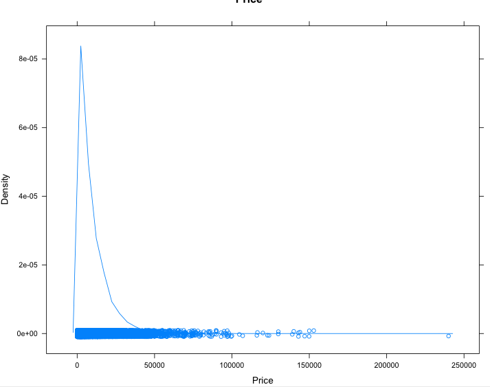
Much better! But we also note several other problems like lots of missing prices in general. These could be corrected one-by- one perhaps. There are also lots of cars for sale at the price of $1. This is a common advertising tactic to post for the minimum price since most people sort prices lowest-to-highest and thus these ads get seen at the top more often. Most of these are misleading ads by dealers, some are for car parts, some are offers for car financing.
> sum( is.na(vehicle$price) )
[1] 3328
> sum( vehicle$price == 1 & !is.na(vehicle$price) )
[1] 612
The same holds for almost all ads less than $500. There is just too much data to clean up manually here so we will exclude them. SURELY we are throwing away some good data here and biasing our results if we are going to erase them out of the data. Fortunately, we can modify filter_high_price function to filter_low_price function.
> filter_low_price = function(maker,year,header,price){
    idx = (vehicle$maker == maker & vehicle$year %in% c(year, year+1) &
          vehicle$price < 100000 & vehicle$price > 1 &
          grepl(pattern = gsub(maker,"",gsub("\\d+\\s","",header), ignore.case=TRUE),x = vehicle$header, ignore.case = TRUE) &
          !is.na(vehicle$maker) & !is.na(vehicle$price) & !is.na(vehicle$header))
  if(length(vehicle$price[idx])!= 0){
    newPrice = round( mean(vehicle$price[idx]), digits = -3)
    if(price < 1.5*newPrice) vehicle$price[vehicle$price == price & !is.na(vehicle$price)] <<- newPrice #return to global environment
  }
}

> idx = which( vehicle$price <= 500 & !is.na(vehicle$price))
> shortlist = vehicle[ idx, c("header", "price", "maker", "year") ]
> sapply(1:length(shortlist$maker), function(i) filter_low_price(shortlist$maker[i],shortlist$year[i],shortlist$header[i], shortlist$price[i]))
[1] Error in if(price < 1.5*newPrice) {: missing Value where TRUE/FALSE needed
Oops! We got error. So I use traceback() command to see where the error is:
> traceback()
4: filter_low_price(shortlist$maker[i], shortlist$year[i], shortlist$header[i],
       shortlist$price[i]) at #1
3: FUN(X[[i]], ...) at #1
2: lapply(X = X, FUN = FUN, ...)
1: sapply(1:length(shortlist$maker), function(i) filter_low_price(shortlist$maker[i],
       shortlist$year[i], shortlist$header[i], shortlist$price[i]))
I guess that there are something wrong with the shortlist data frame. Thanks to RStudio/DT package, we can look at the data more directly.
# install from CRAN
> install.packages('DT')
> idx = which( vehicle$price <= 500 & !is.na(vehicle$price))
> shortlist = vehicle[ idx, c("header", "price", "maker", "year") ]
> datatable(shortlist)
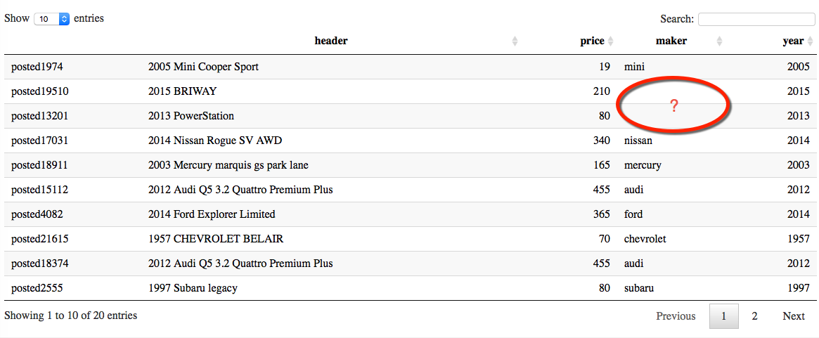
Clearly, some NA values has caused the problem to filter_low_price function, since it doesn’t detect the NA of the maker. So we remove the NA out of shortlist$maker, we will deal with them later.
> idx = which( vehicle$price <= 500 & !is.na(vehicle$price) & !is.na(vehicle$maker))
> shortlist = vehicle[ idx, c("header", "price", "maker", "year") ]
> sapply(1:length(shortlist$maker), function(i) filter_low_price(shortlist$maker[i],shortlist$year[i],shortlist$header[i], shortlist$price[i]))
Let’s check the data frame where the vehicle$price <= 500 to see whether it works:
> idx = which( vehicle$price <= 500 & !is.na(vehicle$price) & !is.na(vehicle$maker))
> vehicle[ idx, c("header", "price", "maker", "year") ]
                                            header price     maker year
posted1974                  2005 Mini Cooper Sport    19      mini 2005
posted17031               2014 Nissan Rogue SV AWD   340    nissan 2014
posted18911      2003 Mercury marquis gs park lane   165   mercury 2003
posted15112  2012 Audi Q5 3.2 Quattro Premium Plus   455      audi 2012
posted4082              2014 Ford Explorer Limited   365      ford 2014
posted21615                  1957 CHEVROLET BELAIR    70 chevrolet 1957
posted18374  2012 Audi Q5 3.2 Quattro Premium Plus   455      audi 2012
posted2555                      1997 Subaru legacy    80    subaru 1997
posted18929             2014 Ford Explorer Limited   365      ford 2014
posted9448                2012 Chrysler 300-Series   179  chrysler 2012
posted29613               1998 ford e150 econoline   375      ford 1998
posted128913                       1992 Saturn SL2    80    saturn 1992
posted229713   1961 chevrolet corvette convertible    53 chevrolet 1961
posted229813   1961 chevrolet corvette convertible    53 chevrolet 1961
posted229913   1961 chevrolet corvette convertible    53 chevrolet 1961
The data frame is much shorter. So, it works! Also we can erase all the data in this data frame because the price of all the entries in this data frame does not make sense and we can find the similar information of them in the vehicle data frame. Let’s erase them:
vehicle = vehicle[-idx,]
> quantile(x = vehicle$price, probs = c(0.05,0.99), na.rm = TRUE)
   5%   99%
 1350 46000
=======================================================================
Price is not the only variable we should care about in this dataset. So let’s check the list of variables again:
> names(vehicle)
 [1] "id"           "title"        "body"         "lat"          "long"
 [6] "posted"       "updated"      "drive"        "odometer"     "type"
[11] "header"       "condition"    "cylinders"    "fuel"         "size"
[16] "transmission" "byOwner"      "city"         "time"         "description"
[21] "location"     "url"          "price"        "year"         "maker"
[26] "makerMethod"
type stands for types of vehicle. List all the different types of vehicle:
> unique(vposts$type)
 [1] coupe       SUV         sedan       hatchback   wagon       van
 [7] <NA>        convertible pickup      truck       mini-van    other
[13] bus         offroad
or we can use table function instead of using unique
> names( table(vehicle$type, useNA = "ifany") )
 [1] "bus"         "convertible" "coupe"       "hatchback"   "mini-van"
 [6] "offroad"     "other"       "pickup"      "sedan"       "SUV"
[11] "truck"       "van"         "wagon"       NA
To make use of the types of vehicle, we must know the proportion of these types of vehicle:
> sort( round( x = prop.table( x = table(vehicle$type, useNA = "ifany") ), digits = 4) )

        bus     offroad    mini-van         van       wagon       other
     0.0006      0.0019      0.0131      0.0146      0.0161      0.0192
convertible   hatchback      pickup       truck       coupe         SUV
     0.0204      0.0236      0.0262      0.0347      0.0469      0.1213
      sedan        <NA>
     0.2031      0.4583
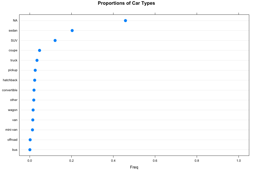
Let’s plot the proportions. I use dotplot from lattice library.
> t = prop.table( x = table(vehicle$type, useNA = "ifany") )
> dotplot(x = sort(t), xlim = c(-0.05, 1.05), cex = 1.5, main = "Proportions of Car Typ
+ es")

We made a mistake! Apparently, NA is missing from the chart. Or we could say that lattice>dotplot does not plot NA at all. So we can force it to do that by:
> names(t)[ is.na(names(t)) ] = "NA"
> t
         bus  convertible        coupe    hatchback     mini-van      offroad
0.0006347008 0.0203681265 0.0469101610 0.0236281807 0.0130690670 0.0019041025
       other       pickup        sedan          SUV        truck          van
0.0192141250 0.0262246841 0.2030754140 0.1213432577 0.0346777451 0.0145981190
       wagon           NA
0.0160983209 0.4582539957

> dotplot(x = sort(t), xlim = c(-0.05, 1.05), cex = 1.5, main = "Proportions of Car Types")
Let’s look at proportions among the non-missing (not NA)
> t = prop.table( x = table(vehicle$type[ !is.na(vehicle$type) ], useNA = "ifany") )
> dotplot(x = sort(t), xlim = c(-0.05, 1.05), cex = 1.5, main = "Proportions of Car Types Among Non-Missing")
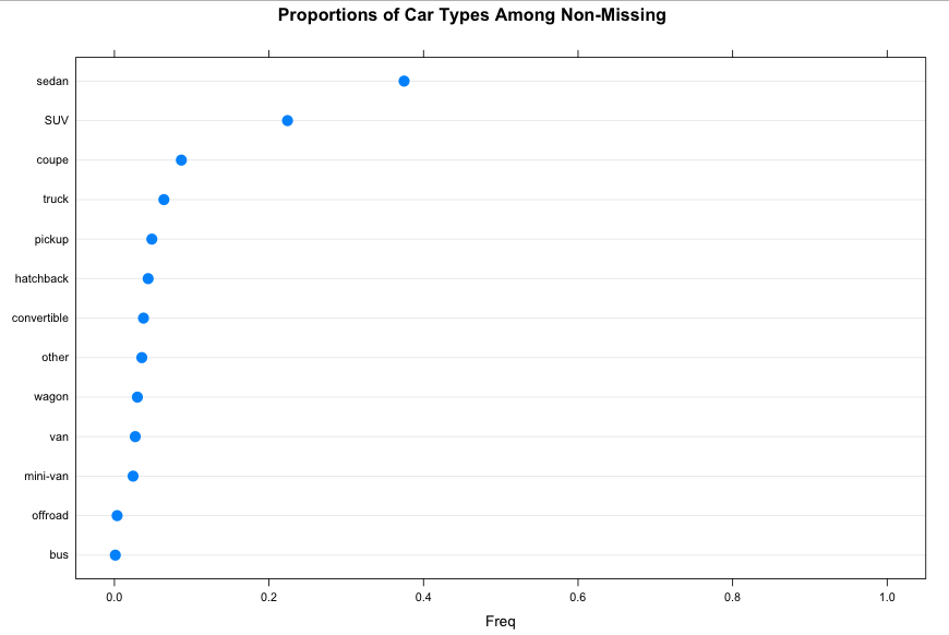
Observed: Nearly half of the data is missing the vehicle type. Among the non-missing type, 40% of the vehicle is sedan.
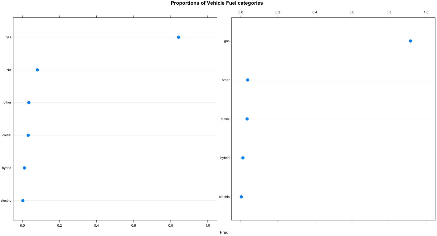
- We are doing the same with
fuel
> t = prop.table( x = table(vehicle$fuel, useNA = "ifany") )
> names(t)[ is.na(names(t)) ] = "NA"
> plot1 = dotplot(x = sort(t), xlim = c(-0.05, 1.05), cex = 1.5, main = "Proportions of Vehicle Fuel categories")
> t = prop.table( x = table(vehicle$fuel[ !is.na(vehicle$fuel) ], useNA = "ifany") )
> plot2 = dotplot(x = sort(u), xlim = c(-0.05, 1.05), cex = 1.5, main = "Proportions of Vehicle Fuel categories Among Non-Missing")
> library(latticeExtra) # It is used to combine lattice plots since par(mfrow) does not work with lattice
> c(plot1,plot2)
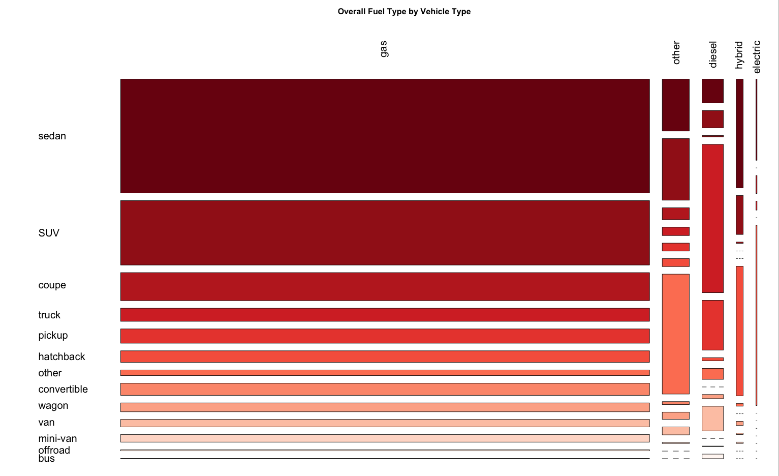
We can display the relationship between fuel type and vehicle type by using mosaic plots
> tbl = table(vehicle$fuel, vehicle$type)
> row.order = order( rowSums( tbl ), decreasing = TRUE )
> col.order = order( colSums( tbl ), decreasing = TRUE )
> tbl = tbl[ row.order, col.order ]
> col.palette = colorRampPalette(brewer.pal(9,"Reds"))(length(col.order))
> mosaicplot(tbl, las = 2, color = rev(col.palette),
+            main =  "Overall Fuel Type by Vehicle Type", cex = 1.5)
Question: Does this depend on transmission type?
> fuelVehicleBytransmission = split( vehicle[ , c("fuel", "type")], vehicle$transmission)
> invisible(
+     lapply( 1:length(fuelVehicleBytransmission), FUN = function(x){
+             tbl = table(fuelVehicleBytransmission[[x]]$fuel, fuelVehicleBytransmission[[x]]$type)
+           row.order = order( rowSums( tbl ), decreasing = TRUE )
+           col.order = order( colSums( tbl ), decreasing = TRUE )
+           tbl = tbl[ row.order, col.order ]
+           # Get color palette and then reverse the order darkest to lightest
+           col.palette = colorRampPalette(brewer.pal(9,"Blues"))(length(col.order))
+           col.palette = col.palette[ length(col.palette):1 ]
+           mosaicplot(tbl, las = 2, color = col.palette,
+                      main = paste0("Fuel and Vehicle by Transmission = ",
+                                    names(fuelVehicleBytransmission)[x]), cex = 1.5
+                      )
+           }
+           )
+         )
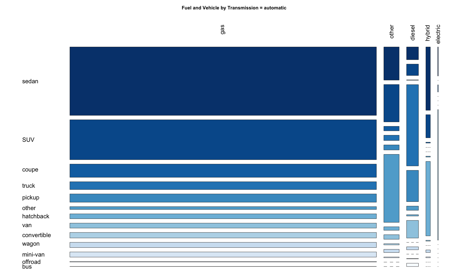
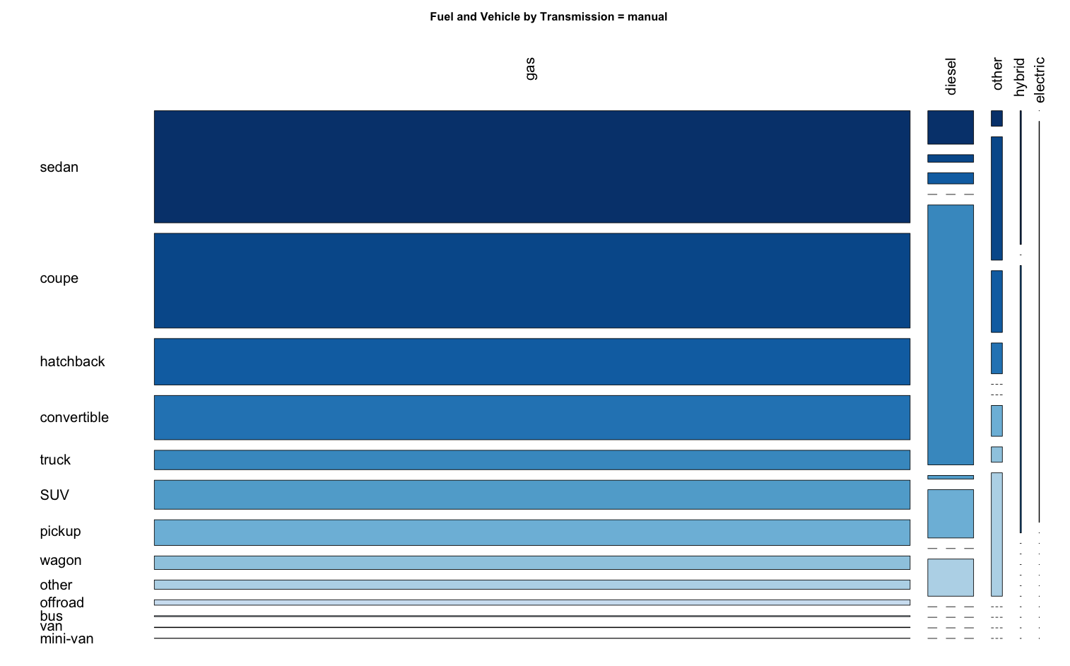
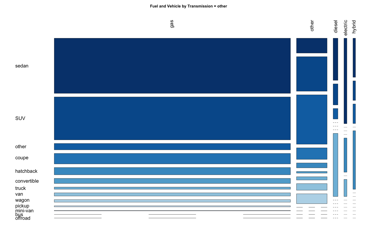
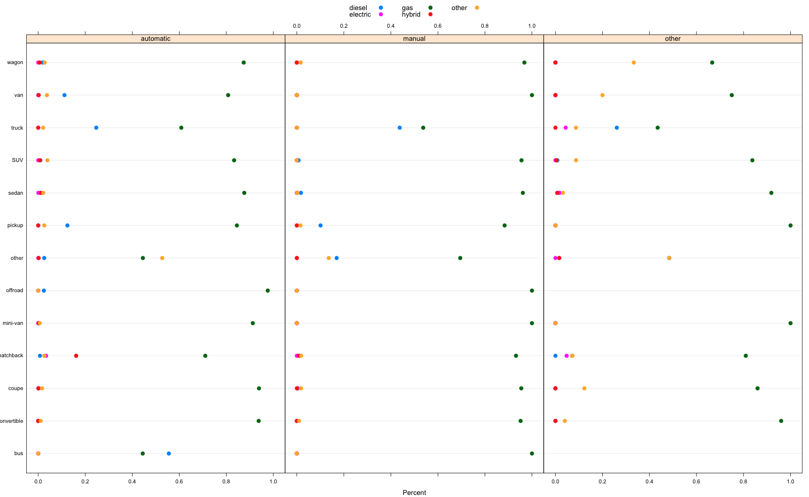
HOWEVER, IT IS HARD TO SEE THIS RELATIONSHIP WITH 3 MOSAIC PLOTs => Use dotplot
> dotplot(
+   prop.table( table(vehicle$type , vehicle$transmission,  vehicle$fuel, useNA = "ifany") ,margin = c(1,2) ),
+ xlim = c(-0.05,1.05), auto.key = list(columns = 3), par.settings = simpleTheme(cex= 1.2, pch = 16),
+ xlab = "Percent"
+ )
-
Instead of focusing about price variable only, we should look at other variables. In these variables, I can think of examining the relationship between byOwner and city.
A. For city variable:
> levels(vehicle$city)
[1] "boston"   "chicago"  "denver"   "lasvegas" "nyc"      "sac"      "sfbay"
> length( levels(vehicle$city) )
[1] 7
> table(vehicle$city)

  boston  chicago   denver lasvegas      nyc      sac    sfbay
    4955     4883     4977     4963     4981     4966     4937
The above table shows us the number of vehicles in different cities.
B. For byOwner variable:
It tells us information about whether the vehicle is listed or sold by owner or dealer. Since it is a TRUE/FALSE vector, we should create another variable with observation as Owner/Dealer. So we call it ownerDealer
library(dplyr)
lut = c("TRUE" = "Owner", "FALSE" = "Dealer")
ownerDealer= (lut[as.character(vehicle$byOwner)] %>% unname())
It is quite suspicious that all cities have roughly 5000 observations and that percentages are almost 50/50. It does not seem right…
> prop.table(table(vehicle$ownerDealer, vehicle$city), margin = 2)

            boston   chicago    denver  lasvegas       nyc       sac     sfbay
  Dealer 0.5025227 0.5097276 0.5005023 0.5015112 0.5005019 0.5000000 0.5013166
  Owner  0.4974773 0.4902724 0.4994977 0.4984888 0.4994981 0.5000000 0.4986834
=======================================================================
Question 6